Activation functions
CReLU
Concatenated ReLU.

Using the CReLU doubles the size of the input to the next layer, increasing the number of parameters. However, Shang et al. showed that CReLU can improve accuracy on image recoginition tasks when used for the lower convolutional layers, even when halving the number of filters in those layers at the same time.
ELU
Exponential Linear Unit.

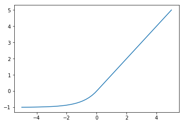
In practice the hyperparameter  is always set to 1.
Compared to ReLUs, ELUs have a mean activation closer to zero which is helpful. However, this advantage is probably nullified by batch normalization.
The more gradual decrease of the gradient should also make them less susceptible to the dying ReLU problem, although they will suffer from the vanishing gradients problem instead.
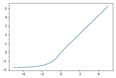
GELU
Gaussian Error Linear Unit. The name comes from the use of the Gaussian error function in the definition:

where  is the CDF of the normal distribution.
It can be approximated as:

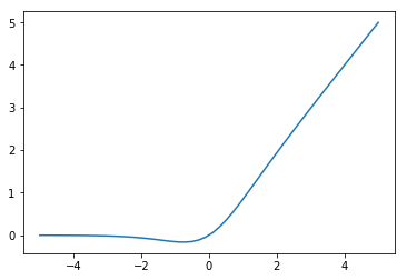
This can be seen as a smoothed version of the ReLU.
Was found to improve performance on a variety of tasks compared to ReLU and ELU (Hendrycks and Gimpel (2016)). The authors speculate that the activation’s curvature and non-monotonicity may help it to model more complex functions.
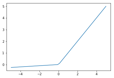
LReLU
Leaky ReLU. Motivated by the desire to have gradients where the ReLU would have none but the gradients are very small and therefore vulnerable to the vanishing gradients problem in deep networks. The improvement in accuracy from using LReLU instead of ReLU has been shown to be very small (Maas et al. (2013)).

 is a fixed hyperparameter, unlike the PReLU. A common setting is 0.01.
Maxout
An activation function designed to be used with dropout.
![f(x) = \max_{j \in [1,k]} x^T W_j + b_j](_images/math/827bcd77f75cfad4b61dce6184a819ed3c9793a3.svg)
where  is a hyperparameter.
Maxout can be a piecewise linear approximation for arbitrary convex activation functions. This means it can approximate ReLU, LReLU, ELU and linear activations but not tanh or sigmoid.
Was used to get state of the art performance on MNIST, SVHN, CIFAR-10 and CIFAR-100.
PReLU
Parametric ReLU.

Where is a learned parameter, unlike in the Leaky ReLU where it is fixed.
Was used to achieve state of the art performance on ImageNet (He et al. (2015)).
ReLU
Rectified Linear Unit. Unlike the sigmoid or tanh activations the ReLU does not saturate which has led to it being widely used in deep networks.

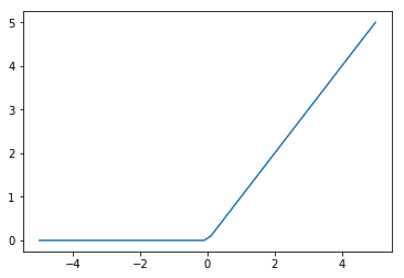
The fact that the gradient is 1 when the input is positive means it does not suffer from vanishing and exploding gradients. However, it suffers from its own ‘dying ReLU problem’ instead.
The Dying ReLU Problem
When the input to a neuron is negative, the gradient will be zero. This means that gradient descent will not update the weights so long as the input remains negative. A smaller learning rate helps solve this problem.
The Leaky ReLU and the Parametric ReLU (PReLU) attempt to solve this problem by using  where a is a small constant like 0.1. However, this small gradient when the input in negative means vanishing gradients are once again a problem.
SELU
Scaled Exponential Linear Unit.

Where  and are hyperparameters, set to
  and
and  .
.
The SELU is designed to be used in networks composed of many fully-connected layers, as opposed to CNNs or RNNs, the principal difference being that CNNs and RNNs stabilize their learning via weight sharing. As with batch normalization, SELU activations give rise to activations with zero mean and unit variance but without having to explicitly normalize.
The ELU is a very similar activation. The only difference is that it has  and
and  .
.
Initialisation
Klambauer et al. (2017) recommend initialising layers with SELU activations according to  where
where  are the parameters for layer
  of the network and
  is the size of layer of the network.
Dropout
Instead of randomly setting units to zero as in conventional dropout, the authors propose setting units to  where and are the hyperparameters given previously. They refer to this as alpha dropout.
Sigmoid
Activation function that maps outputs to be between 0 and 1.

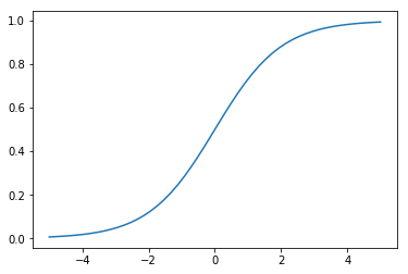
Has problems with saturation. This makes vanishing and exploding gradients a problem and initialization extremely important.
Softmax
All entries in the output vector are in the range (0,1) and sum to 1, making the result a valid probability distribution.

Where  is a vector of length
  . This vector is often referred to as the logit.
Unlike most other activation functions, the softmax does not apply the same function to each item in the input independently. The requirement that the output vector sums to 1 means that if one of the inputs is increased the others must decrease in the output.
The Softmax Bottleneck
A theorised problem that occurs when using the softmax to predict the next token in language modeling. It views language modeling as a matrix factorization problem:

Where  is the contexts,
  are the word vectors and
  are the conditional probabilities for words given contexts. The vast number of contexts in language means that the matrix is almost certainly high rank and so the dimensionality of the word embeddings is probably not sufficient to solve the matrix factorization problem adequately.
Mixture of Softmaxes
Mixture model intended to avoid the Softmax Bottleneck.
The probability of a word given some context  is the weighted average of softmax distributions:

where  is the weight of component .
Softplus
Activation whose output is bounded between 0 and infinity, making it useful for modeling quantities that should never be negative such as the variance of a distribution.

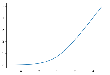
Unlike the ReLU, gradients can pass through the softmax when  .
.
Tanh
Activation function that is used in the GRU and LSTM. It is between -1 and 1 and centered around 0, unlike the sigmoid.

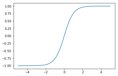
Has problems with saturation like the sigmoid. This makes vanishing and exploding gradients a problem and initialization extremely important.