Loss functions
For classification problems,  is equal to 1 if the example is a positive and 0 if it is a negative.
  can take on any value (although predicting outside of the (0,1) interval is unlikely to be useful).
Classification
Cross-entropy loss
Loss function for classification.

where c are the classes.  equals 1 if example
  is in class
  and 0 otherwise.
  is the predicted probability that example is in class .
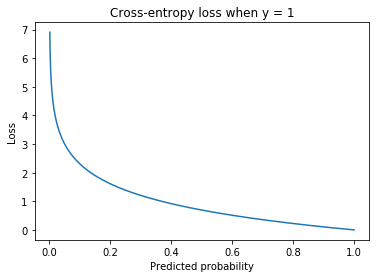
For discrete distributions (ie classification problems rather than regression) this is the same as the negative log-likelihood loss.
Hinge loss
Let positives be encoded as  and negatives as
  . Then the hinge loss is defined as:

The margin  is a hyperparameter that is commonly set to 1.
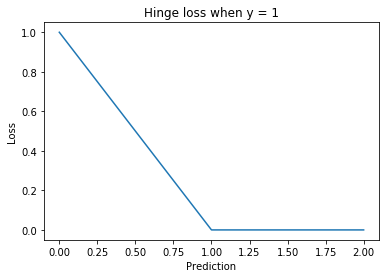
Used for training SVMs.
Focal loss
Variant of the cross-entropy loss, designed for use on datasets with severe class imbalance. It is defined as:

Where  is a hyperparameter that determines the relative importance of the classes. If
  the focal loss is equivalent to the cross-entropy loss.
Noise Contrastive Estimation
Like negative sampling, this is a technique for efficient learning when the number of output classes is large. Useful for language modelling.
A binary classification task is created to disambiguate pairs that are expected to be close to each other from ‘noisy’ examples put together at random.
In essence, rather than estimating  , NCE estimates
  where
where  if has been sampled from the real distribution and
  if has been sampled from the noise distribution.
NCE makes training time at the output layer independent of the number of classes. It remains linear in time at evaluation, however.

 is a hyperparameter, denoting the number of noise samples for each real sample.
  is a label sampled from the data distribution and
  is one sampled from the noise distribution.
  if the pair
  was drawn from the data distribution and 0 otherwise.
Embeddings
Contrastive loss
Loss function for learning embeddings, often used in face verification.
The inputs are pairs of examples  and
and  where if the two examples are of the similar and
  if not.

Where and are the embeddings for the two examples and is a hyperparameter called the margin.  is a distance function, usually the Euclidean distance.
Intuition
If the two examples and are similar and we want to minimize the distance  . Otherwise (
 ) we wish to maximize it.
The margin
If we want to make as large as possible to minimize the loss. However, beyond the threshold for classifying the example as a negative increasing this distance will not have any effect on the accuracy. The margin ensures this intuition is reflected in the loss function. Using the margin means increasing beyond has no effect.
There is no margin for when . This case is naturally bounded by 0 as the Euclidean distance cannot be negative.
Negative sampling
The problem is reframed as a binary classification problem.

where  and are two examples,
  is the learned embedding function and if the pair
  are expected to be similar and otherwise. The dot product measures the distance between the two embeddings.
Noise Contrastive Estimation
A binary classification task is created to disambiguate pairs that are expected to be close to each other from ‘noisy’ examples put together at random.

where and are two examples, is the learned embedding function and if the pair are expected to be similar and if not (because they have been sampled from the noise distribution). The dot product measures the distance between the two embeddings and the sigmoid function transforms it to be between 0 and 1 so it can be interpreted as a prediction for a binary classifier.
This means maximising the probability that actual samples are in the dataset and that noise samples aren’t in the dataset. Parameter update complexity is linear in the size of the vocabulary. The model is improved by having more noise than training samples, with around 15 times more being optimal.
Triplet loss
Used for training embeddings with triplet networks. A triplet is composed of an anchor ( ), a positive example (
 ) and a negative example (
 ). The positive examples are similar to the anchor and the negative examples are dissimilar.

Where is a hyperparameter called the margin. is a distance function, usually the the Euclidean distance.
The margin
We want to minimize  and maximize
  . The former is lower-bounded by 0 but the latter has no upper bound (distances can be arbitrarily large). However, beyond the threshold to classify a pair as a negative, increasing this distance will not help improve the accuracy, a fact which needs to be reflected in the loss function. The margin does this by ensuring that there is no gain from increasing beyond
  since the loss will be set to 0 by the maximum.
Regression
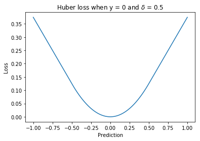
Huber loss
A loss function used for regression. It is less sensitive to outliers than the squared loss since there is only a linear relationship between the size of the error and the loss beyond  .
.

Where is a hyperparameter.
Squared loss
A loss function used for regression.

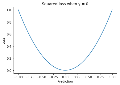
Disadvantages
The squaring means this loss function weights large errors more than smaller ones, relative to the magnitude of the error. This can be particularly harmful in the case of outliers. One solution is to use the Huber loss.