Gaussian processes¶

Gaussian processes model a probability distribution over functions.

Let $f(x)$ be some function mapping vectors to vectors. Then we can write:

$f(x) \sim GP(m(x),k(x,x'))$

where $m(x)$ represents the mean vector:

$m(x) = \mathbb{E}[f(x)]$

and $k(x,x')$ is the kernel function.

Kernel function¶

The kernel is a function that represents the covariance function for the Gaussian process.

$k(x,x') = \text{Cov}(f(x),f(x'))$

$k(x,x') = \mathbb{E}[(f(x) - m(x))(f(x') - m(x'))^T]$

The kernel can be thought of as a prior for the shape of the function, encoding our expectations for the amount of smoothness or non-linearity.

Not all conceivable kernels are valid. The kernel must produce covariance matrices that are positive-definite.

Linear kernel¶

$k(x,x') = x \cdot x'$

Some functions sampled from a Gaussian process with a linear kernel:

_images/linear.png

Polynomial kernel¶

$k(x,x';a,b) = (x \cdot x' + a)^b$

Functions sampled from a Gaussian process with a polynomial kernel where $a=1$ and $b=2$ :

_images/polynomial_2.png

Gaussian kernel¶

Also known as the radial basis function or RBF kernel.

$k(x,x'; \sigma, l) = \sigma_2 \exp(-\frac{{(x - x')}_2}{2l^2})$

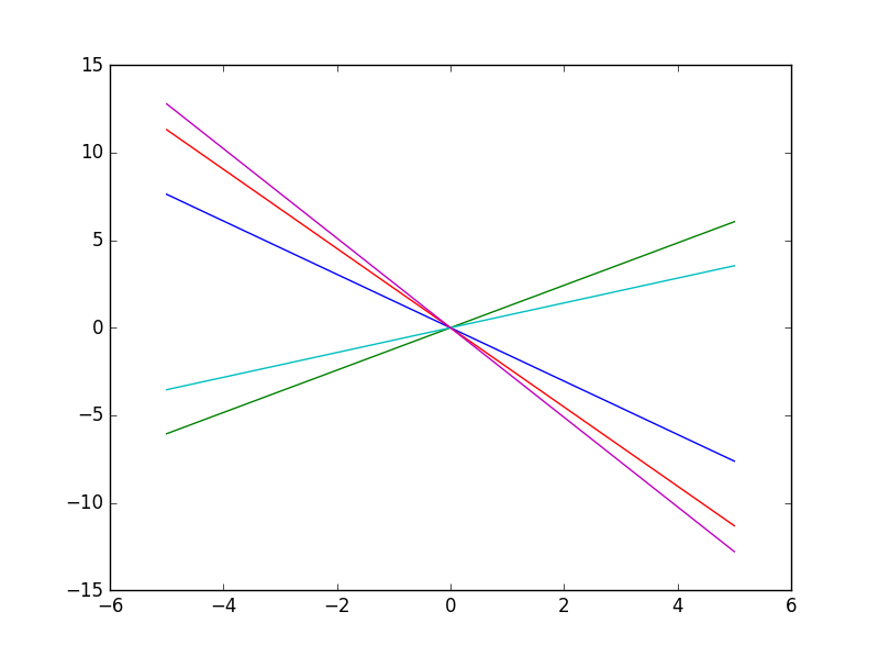
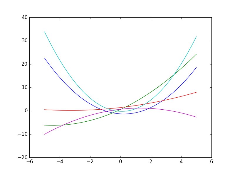
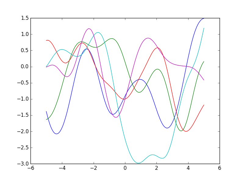
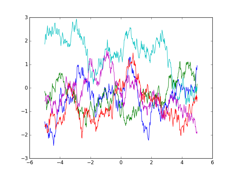
Some functions sampled from a GP with a Gaussian kernel:

_images/gaussian.png

Laplacian kernel¶

$k(x,x') = \exp(-|x - x'|)$

Functions sampled from a GP with a Laplacian kernel:

_images/laplace.png

Sampling from a Gaussian process¶

The method is as follows:

Decide on a vector of inputs $x$ for which we want to compute $f(x)$ , where $f$ is some function which we will sample from the Gaussian process.
Compute the matrix $K$ where $K_{ij} = k(x_i,x_j)$ .
Perform Cholesky decomposition on $K$ , yielding a lower triangular matrix $L$ .
Sample a vector of numbers from a standard Gaussian distribution, $s_i \sim N(0, 1)$ .
Take the dot product of $L$ and the vector $s$ to get the samples $f(x) = L \cdot s$ .