Generative networks
Models the joint distribution over the features  , ignoring any labels.
The model can be estimated by trying to maximise the probability of the observations given the parameters. However, this can be close to intractable for cases like images where the number of possible outcomes is huge.
Autoencoders
A network for dimensionality reduction that can also be used for generative modelling.
In its simplest form, an autoencoder takes the original input (eg the pixel values of an image) and transforms them into a hidden layer with fewer features than the original. This ‘bottleneck’ means a compressed representation of the input. The part of the network which does this transformation is known as the encoder. The second part of an autoencoder is the decoder which takes the bottleneck layer and uses it to try and reconstruct the original input. This part is known as the decoder.
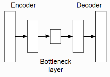
Autoencoders can be used as generative networks by sampling a new hidden state in the bottleneck layer and running it through the decoder.
Convolutional autoencoders
An autoencoder composed of standard convolutional layers and upsampling layers rather than fully connected layers.
Denoising Autoencoder (DAE)
Adds noise to prevent the hidden layer(s) from learning the identity function. This is particularly useful when the width of the narrowest hidden layer is at least as wide as the input layer.
Variational Autoencoder (VAE)
Unlike the standard autoencoder, the VAE can take noise as an input and use it to generate a sample from the distribution being modelled. ‘Variational’ refers to the Variational Bayes method which is used to approximate the true objective function with one that is more computable.
In order to modify the standard autoencoder to allow sampling, the distribution of the encoded image vectors is constrained to be roughly Normal(0,1). This means sampling can be done by sampling a random vector from N(0,1) and running the decoder on it.
There are two vectors outputted by the encoder, one for the mean and one for the variance. The closeness of these vectors to the unit Gaussian is measured by the KL-divergence.
The total loss is the sum of the reconstruction loss (mean squared error) and the KL-divergence:

where  and
and  are the mean and standard deviation of the encoding.
Evidence-lower bound (ELBO)
A lower bound on the log probability of the data given the parameters. In a VAE this function is maximised instead of the true likelihood.
Reparameterization trick
A method for backpropagating through nodes in the graph that have random sampling. Suppose the first half of a network outputs and . We want to sample from the distribution they define and then compute the loss function on that sample.
We can rewrite  as
as  where
where  . This means the gradients no longer have to go through stochastic nodes in the graph.
Problems
- The use of the mean squared error means the network tends to produce blurry images. A GAN does not have this problem.
- The assumption of independence in the entries of the hidden vector may also contribute to poor results.
Autoregressive Networks
Unlike other generative models such as GANs or VAEs, these models generate their results sequentially. At each timestep they compute  . The process is broadly the same as generating a sample of text using an RNN but can be used to generate images.
Autoregressive networks exploit the chain rule to express the joint probability as the product of conditional probabilities:

PixelRNN
The model reads the image one pixel at a time and row by row, form the top left to the bottom right. Their best model used a 7 layer diagonal bidirectional LSTM with residual connections between the layers to ease training.
Pixels are modelled as being drawn from a discrete distribution with 256 values. The model has one 256-way output layer for each colour channel. When reading in the pixels, colour channels are handled sequentially so that the red channel is conditioned only on the previous pixels, the blue channel can use the red as well as the previous pixels and the green can use both the blue and red.
PixelCNN
PixelCNN was also proposed in van den Oord et al. (2016) but the results were not as good as PixelRNN.
PixelCNN++ improves upon PixelCNN with a number of modifications, improving upon both it and PixelRNN. The modifications are:
- The 256-way softmax for each colour channel is replaced by a mixture of logistic distributions. This requires two parameters and one weight for each distribution, making it much more efficient given that only around 5 distributions are needed. The edge cases of 0 and 255 are handled specially.
- “Conditioning on whole pixels”
- Convolutions with a stride of 2 are used to downsample the image and effective increase the size of the convolutions’ receptive fields.
- Residual connections are added between the convolutional layers. These help to prevent information being lost through the downsampling.
- Dropout is added on the model’s residual connection to improve generalization.
WaveNet
Energy-based Models
Also known as Undirected Graphical Models.
An energy function models the probability density. A model is learnt that minimises the energy for correct combinations of the variables and maximises it for incorrect ones. This function is minimised during inference.
The loss function is minimised during training. The energy function is a component of it.
Generative Adversarial Network (GAN)
Unsupervised, generative image model. A GAN consists of two components; a generator, G which converts random noise into images and a discriminator, D which tries to distinguish between generated and real images. Here, ‘real’ means that the image came from the training set of images in contrast to the generated fakes.
Problems
- The training process can be unstable when trained solely with the adversarial loss as G can create images to confuse D that are not close to the actual image distribution. D will then learn to discriminate amongst these samples, causing G to create new confusing samples. This problem can be addressed by adding an L2 loss which penalizes a lack of similarity with the input distribution.
- Mode collapse. This is when the network stops generating certain classes (or more generally, modes). For example, it may only create 6’s on MNIST.
- There is no way of telling how well it is doing except by manually inspecting the image outputs. This makes comparing different approaches difficult and early stopping impossible.
Notable variants
- A Style-Based Generator Architecture for Generative Adversarial Networks, Karras et al. (2018)
- Progressive Growing of GANs for Improved Quality, Stability, and Variation, Karras et al. (2017)
- Unpaired Image-to-Image Translation using Cycle-Consistent Adversarial Networks, Zhu et al. (2017)
- BEGAN: Boundary Equilibrium Generative Adversarial Networks, Berthelot et al. (2017) - Gets similar quality results as the WGAN-GP.
- Improved Training of Wasserstein GANs, Gulrajani et al. (2017)
- Wasserstein GAN, Arjovsky et al. (2017) - Replaces the original loss function, improving stability. The WGAN-GP (2017) is a further improved version.
- InfoGAN: Interpretable Representation Learning by Information Maximizing Generative Adversarial Nets, Chen et al. (2016) - Is able to disentangle various aspects like pose vs lighting and digit shape vs writing style.
- Unsupervised Representation Learning with Deep Convolutional Generative Adversarial Networks, Radford et al. (2015) - Has a number of architectural improvements over the original GAN but is not fundamentally different.