Optimization
Automatic differentiation
Has two distinct modes - forward and reverse.
Forward mode takes an input to the graph and evaluates the derivative of all subsequent nodes with respect to it.
Reverse mode takes an output (eg the loss) and differentiates it with respect to all inputs. This is usually more useful in neural networks since it can be used to get the derivatives for all the parameters in one pass.
Backpropagation
Naively summing the product of derivatives over all paths to a node is computationally intractable because the number of paths increases exponentially with depth.
Instead, the sum over paths is calculated by merging paths back together at the nodes. Derivatives can be computed either forward or backward with this method.
Backpropagation through time (BPTT)
Used to train RNNs. The RNN is unfolded through time.
When dealing with long sequences (hundreds of inputs), a truncated version of BPTT is often used to reduce the computational cost. This stops backpropagating the errors after a fixed number of steps, limiting the length of the dependencies that can be learned.
Batch size
Pros of large batch sizes:
- Decreases the variance of the updates, making convergence more stable. From this perspective, increasing the batch size has very similar effects to decreasing the learning rate.
- Matrix computation is more efficient.
Cons of large batch sizes:
- Very large batch sizes may not fit in memory.
- Smaller number of updates for processing the same amount of data, slowing training.
- Hypothesized by Keskar et al. (2016) to have worse generalization performance since they result in sharper local minima being reached.
Curriculum learning
Training the classifier with easy examples initially and gradually transitioning to the harder ones. Useful for architectures which are very hard to train.
Depth
Depth increases the representational power of a network exponentially, for a given number of parameters. However, deeper networks can also be considerably harder to train, due to vanishing and exploding gradients or dying ReLUs. Problems stemming from depth are seen both in deep feedforward networks and in recurrent networks, where the depth comes from being unfolded over a large number of timesteps.
Potential solutions include:
- Using a smaller learning rate
- Skip connections
- Batch normalization
- Memory cells. Used in the Neural Turing Machine for learning long dependencies.
- Auxiliary loss functions (eg Szegedy et al. (2016))
- Orthogonal initialization
Distributed training
Training a neural network using multiple machines in parallel. Unfortunately gradient descent is a naturally sequential process since each iteration uses the parameters from the previous one. This means distributed training requires algorithms written specifically for that purpose.
Distributed training methods are broadly classified as being either synchronous or asynchronous, more details of which are given in their sections below.
Asynchronous SGD
Each worker processes a batch of data and computes the gradients. A central server holds the model parameters. The workers fetch the parameters from the parameter server and use them to compute gradients, which are then sent to the parameter server so the weights can be updated.
It is likely that while a worker is computing gradients other worker(s) have already finished their gradients and used them to update the parameters. Therefore the update can be several steps out-of-date when the gradient is finally computed. This problem is more severe the more workers there are.
Synchronous SGD
Gradients are accumulated from the workers and summed before updating the network parameters.
Parameter updates can only occur once all the workers have computed their gradients which can slow down learning, unlike in asynchronous SGD. The whole system is limited to the speed of the lowest worker.
Means using larger batch sizes. This could be counteracted by reducing the batch sizes on each of the workers but this would reduce efficiency.
Early stopping
Halting training when the validation loss has stopped decreasing but the training loss is still going down.
End-to-end
The entire model is trained in one process, not as separate modules. For example, a pipeline consisting of object recognition and description algorithms that are trained individually would not be trained end-to-end.
Epoch
A single pass through the training data.
Error surface
The surface obtained by plotting the weights of the network against the loss. For a linear network with a squared loss function, the surface is a quadratic bowl.
Exploding gradient problem
When the gradient grows exponentially as we move backward through the layers.
Gradient clipping can be an effective antidote.
Gradient clipping
Used to avoid exploding gradients in very deep networks by normalizing the gradients of the parameter vector. Clipping can be done either by value or by norm.

 are hyperparameters.
Clipping by norm

Where  is the gradient of the parameter
  and
and  is a hyperparameter.
On the difficulty of training recurrent neural networks, Pascanu et al. (2012)
Learning rate
Pros of large learning rates:
- Training is faster if the large learning rate does not cause problems.
- Lowers the risk of overfitting.
Cons of large learning rates:
- Increases the risk of oscillations during training, especially when not using an optimizer with a momentum term.
- Can make it harder to train deeper networks.
Learning rate decay
Also known as learning rate annealing. Changing the learning rate throughout the training process according to some schedule.
Cosine learning rate decay
The learning rate decays according to a cosine function but is reset to its maximum value once its minimum is reached. The equation for the learning rate at epoch  is:
is:

where  is the number of epochs between warm restarts and
  is the number of epochs that have been performed since the last warm restart. The learning rate fluctuates between
  and
and  .
.
Multiplying by  after every restart was found to increase performance.
The graph below shows cosine learning rate decay with  ,
,  ,
,  and
and  :
:
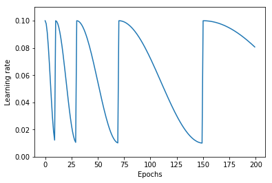
Was shown (Loschilov and Hutter (2016)) to increase accuracy on CIFAR-10 and CIFAR-100 compared to the conventional approach of decaying the learning rate monotonically with a step function.
Note that warm restarts can temporarily make the model’s performance worse. The best model can usually be found when the learning rate is at its minimum.
The following Python code shows how to implement cosine learning rate decay:
t_i = 10 # number of epochs between warm restarts.
t_mult = 2 # double t_i at every restart. set to 1 to ignore.
t_cur = 0 # how many epochs have been performed since the last restart.

min_lr = 0.01
max_lr = 0.1

for epoch in range(num_epochs):
    # warm restart
    if epoch > 0 and t_cur == t_i:
        t_cur = 0
        t_i *= t_mult

    lr = min_lr + 0.5 * (max_lr - min_lr) * (1 + np.cos(np.pi * t_cur / t_i))
    t_cur += 1
Momentum
Adds a fraction of the update from the previous time step to the current time step. The parameter update at time t is given by:


Deep architectures often have deep ravines in their landscape near local optimas. They can lead to slow convergence with vanilla SGD since the negative gradient will point down one of the steep sides rather than towards the optimum. Momentum pushes optimization to the minimum faster. Commonly set to 0.9.
Optimizers
AdaDelta
AdaDelta is a gradient descent based learning algorithm that adapts the learning rate per parameter over time. It was proposed as an improvement over AdaGrad, which is more sensitive to hyperparameters and may decrease the learning rate too aggressively.
AdaGrad
Adam
Adam is an adaptive learning rate algorithm similar to RMSProp, but updates are directly estimated using EMAs of the first and uncentered second moment of the gradient. Designed to combine the advantages of RMSProp and AdaGrad. Does not require a stationary objective and works with sparse gradients. Is invariant to the scale of the gradients.
Has hyperparameters  ,
,  ,
,  and
and  .
.
The biased first moment (mean) estimate at iteration :

The biased second moment (variance) estimate at iteration :

Bias correction for the first and second moment estimates:


The bias correction terms counteracts bias caused by initializing the moment estimates with zeros which makes them biased towards zero at the start of training.
Update the parameters of the network:

This can be interpreted as a signal-to-noise ratio, with the step-size increasing when the signal is higher, relative to the noise. This leads to the step-size naturally becoming smaller over time. Using the square root for the variance term means it can be seen as computing the EMA of  . This reduces the learning rate when the gradient is a mixture of positive and negative values as they cancel out in the EMA to produce a number closer to 0.
Averaged SGD (ASGD)
Runs like normal SGD but replaces the parameters with their average over time at the end.
BFGS
Iterative method for solving nonlinear optimization problems that approximates Newton’s method. BFGS stands for Broyden–Fletcher–Goldfarb–Shanno. L-BFGS is a popular memory-limited version of the algorithm.
Conjugate gradient
Iterative algorithm for solving SLEs where the matrix is symmetric and positive-definite.
Coordinate descent
Minimizes a function by adjusting the input along only one dimension at a time.
Krylov subspace descent
Second-order optimization method. Inferior to SGD.
Natural gradient
At each iteration attempts to perform the update which minimizes the loss function subject to the constraint that the KL-divergence between the probability distribution output by the network before and after the update is equal to a constant.
Revisiting natural gradient for deep networks, Pascanu and Bengio (2014)
Newton’s method
An iterative method for finding the roots of an equation,  . An initial guess (
 ) is chosen and iteratively refined by computing
  .
.

Applied to gradient descent
In the context of gradient descent, Newton’s method is applied to the derivative of the function to find the points where the derivative is equal to zero (the local optima). Therefore in this context it is a second order method.
 where
where  is the inverse of the Hessian matrix at iteration
  .
.
Picks the optimal step size for quadratic problems but is also prohibitively expensive to compute for large models due to the size of the Hessian matrix, which is quadratic in the number of parameters of the network.
Nesterov’s method
Attempts to solve instabilities that can arise from using momentum by keeping the history of previous update steps and combining this with the next gradient step.
RMSProp
Similar to Adagrad, but introduces an additional decay term to counteract AdaGrad’s rapid decrease in the learning rate. Divides the gradient by a running average of its recent magnitude. 0.001 is a good default value for the learning rate ( ) and 0.9 is a good default value for . The name comes from Root Mean Square Propagation.

http://www.cs.toronto.edu/~tijmen/csc321/slides/lecture_slides_lec6.pdf
http://ruder.io/optimizing-gradient-descent/index.html#rmsprop
Subgradient method
A class of iterative methods for solving convex optimization problems. Very similar to gradient descent except the subgradient is used instead of the gradient. The subgradient can be taken even at non-differentiable kinks in a function, enabling convergence on these functions.
Polyak averaging
The final parameters are set to the average of the parameters from the last n iterations.
Saddle points
A point on a function which is not a local or global optimum but where the derivatives are zero.
Gradients around saddle points are close to zero which makes learning slow. The problem can be partially solved by using a noisy estimate of the gradient, which SGD does implicitly.
Saturation
When the input to a neuron is such that the gradient is close to zero. This makes learning very slow. This is a common problem for sigmoid and tanh activations, which saturate for inputs that are too high or too low.
Vanishing gradient problem
The gradients of activation functions like the sigmoid are all between 0 and 1. When gradients are computed via the chain rule they become smaller, increasingly so towards the beginning of the network. This means the affected layers train slowly.
If the gradients are larger than 1 this can cause the exploding gradient problem.
See also the dying ReLU problem.